Exercise 3: electron vs gamma separation
1. Introduction
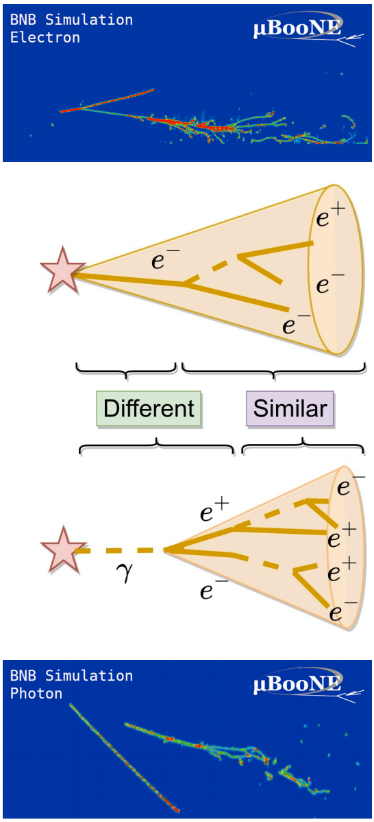
Fig. 14 Difference between an electron vs photon is at the start of the electromagnetic shower, where the photon has a gap. From Wouter Van De Pontseele, ICHEP 2020.
Electrons are visible in a LArTPC detector because of the electromagnetic showers that they trigger.
Photons, on the other hand, are neutral (no charge) and thus remain invisible to the LArTPC eyes until they convert into electrons (pair production) or Compton scatter. In both cases, the visible outcome will be an electromagnetic shower.
How can we differentiate the two, then? The answer is in the very beginning of the EM shower. For an electron, this shower will be topologically connected to the interaction vertex where the electron was produced. For a photon, there will be a gap (equal to the photon travel path) until the EM shower start (when the photon becomes indirectly visible through pair production or Compton scatter). That seems simple enough, right? Wrong, of course.
Energetic photons could interact at a distance short enough from the interaction vertex, that we would not be able to see the gap. Or, the hadronic activity might be invisible, because it includes neutral particles or because the particles are too low energy to be seen. In that case the interaction vertex might be hard to identify, and the notion of a gap goes away too. For such cases, fortunately, there is another way to tell electrons from gamma showers. Another major difference is in the energy loss rate at the start of the EM shower. An electron would leave ionization corresponding to a single ionizing particle, whereas a pair of electron + positron coming from a photon pair production would add up to two ionizing particle. Thus, we expect the dE/dx at the beginning of the shower to be roughly twice larger in the case of a gamma-induced shower compared to an electron-induced shower.
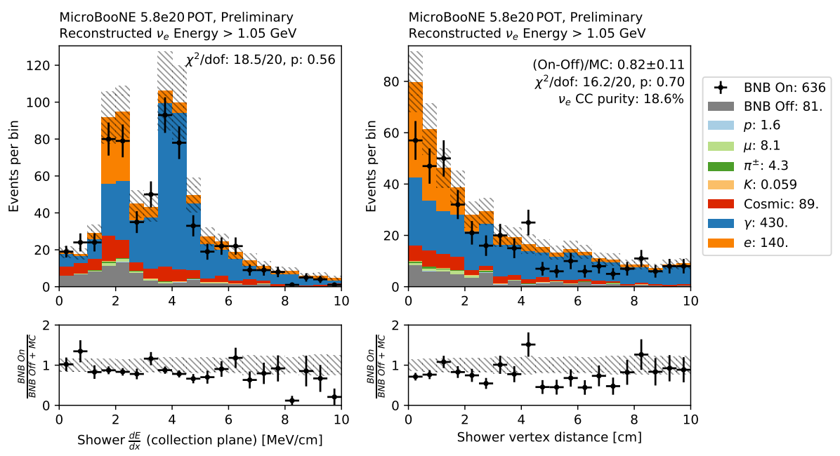
Fig. 15 Example from MicroBooNE. Left is the shower \(dE/dx\), right is the gap between the vertex and shower start. From Wouter Van De Pontseele, ICHEP 2020.
Why do we care? The difference becomes significant if, for example, you are looking for electron neutrinos. One of the key signatures you would be looking for are electrons.
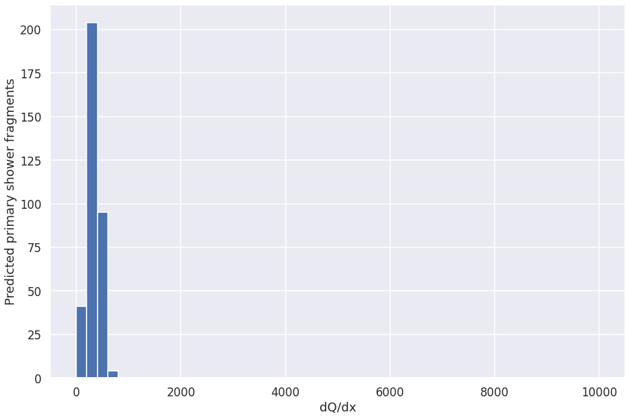
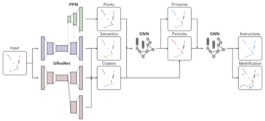
In this exercise, we will focus on finding the start of EM showers and computing the reconstructed dQ/dx in these segments. Optionally, you could compare that to the result of using automatic PID as predicted by the chain.
2. Setup
a. Software and data directory
import os, sys
SOFTWARE_DIR = '%s/lartpc_mlreco3d' % os.environ.get('HOME')
DATA_DIR = os.environ.get('DATA_DIR')
# Set software directory
sys.path.append(SOFTWARE_DIR)
b. Numpy, Matplotlib, and Plotly for Visualization and data handling.
import numpy as np
import matplotlib.pyplot as plt
import seaborn
seaborn.set(rc={
'figure.figsize':(15, 10),
})
seaborn.set_context('talk')
import plotly
import plotly.graph_objs as go
from plotly.subplots import make_subplots
from plotly.offline import download_plotlyjs, init_notebook_mode, plot, iplot
init_notebook_mode(connected=False)
c. MLRECO specific imports for model loading and configuration setup
from mlreco.main_funcs import process_config, prepare
import warnings, yaml
warnings.filterwarnings('ignore')
cfg = yaml.load(open('%s/inference.cfg' % DATA_DIR, 'r').read().replace('DATA_DIR', DATA_DIR),Loader=yaml.Loader)
process_config(cfg, verbose=False)
/usr/local/lib/python3.8/dist-packages/MinkowskiEngine/__init__.py:36: UserWarning:
The environment variable `OMP_NUM_THREADS` not set. MinkowskiEngine will automatically set `OMP_NUM_THREADS=16`. If you want to set `OMP_NUM_THREADS` manually, please export it on the command line before running a python script. e.g. `export OMP_NUM_THREADS=12; python your_program.py`. It is recommended to set it below 24.
Config processed at: Linux ampt017 3.10.0-1160.42.2.el7.x86_64 #1 SMP Tue Sep 7 14:49:57 UTC 2021 x86_64 x86_64 x86_64 GNU/Linux
$CUDA_VISIBLE_DEVICES="0"
d. Initialize and load weights to model using Trainer.
# prepare function configures necessary "handlers"
hs = prepare(cfg)
dataset = hs.data_io_iter
Welcome to JupyROOT 6.22/09
Loading file: /sdf/home/l/ldomine/lartpc_mlreco3d_tutorials/book/data/mpvmpr_062022_test_small.root
Loading tree sparse3d_reco
Warning in <TClass::Init>: no dictionary for class larcv::EventNeutrino is available
Warning in <TClass::Init>: no dictionary for class larcv::NeutrinoSet is available
Warning in <TClass::Init>: no dictionary for class larcv::Neutrino is available
Loading tree sparse3d_reco_chi2
Loading tree sparse3d_reco_hit_charge0
Loading tree sparse3d_reco_hit_charge1
Loading tree sparse3d_reco_hit_charge2
Loading tree sparse3d_reco_hit_key0
Loading tree sparse3d_reco_hit_key1
Loading tree sparse3d_reco_hit_key2
Loading tree sparse3d_pcluster_semantics_ghost
Loading tree cluster3d_pcluster
Loading tree particle_pcluster
Loading tree particle_mpv
Loading tree sparse3d_pcluster_semantics
Loading tree sparse3d_pcluster
Loading tree particle_corrected
Found 101 events in file(s)
Shower GNN: True
Track GNN: True
Particle GNN: False
Interaction GNN: True
Kinematics GNN: False
Cosmic GNN: False
Since one of the GNNs are turned on, process_fragments is turned ON.
Fragment processing is turned ON. When training CNN models from
scratch, we recommend turning fragment processing OFF as without
reliable segmentation and/or cnn clustering outputs this could take
prohibitively large training iterations.
Shower GNN: True
Track GNN: True
Particle GNN: False
Interaction GNN: True
Kinematics GNN: False
Cosmic GNN: False
Since one of the GNNs are turned on, process_fragments is turned ON.
Fragment processing is turned ON. When training CNN models from
scratch, we recommend turning fragment processing OFF as without
reliable segmentation and/or cnn clustering outputs this could take
prohibitively large training iterations.
Freezing 82 weights for a sub-module ppn
Freezing 141 weights for a sub-module uresnet_lonely
Freezing 141 weights for a sub-module uresnet_deghost
Freezing 146 weights for a sub-module graph_spice
Freezing 120 weights for a sub-module grappa_track
Freezing 120 weights for a sub-module grappa_shower
Restoring weights for from /sdf/home/l/ldomine/lartpc_mlreco3d_tutorials/book/data/weights_full_mpvmpr_062022.ckpt...
Done.
Let’s load one iteration worth of data into our notebook:
data, result = hs.trainer.forward(dataset)
Deghosting Accuracy: 0.9830
Segmentation Accuracy: 0.9900
PPN Accuracy: 0.8843
Clustering Accuracy: 0.2691
Clustering Edge Accuracy: 0.1252
Shower fragment clustering accuracy: 0.9581
Shower primary prediction accuracy: 0.9434
Track fragment clustering accuracy: 0.9937
Interaction grouping accuracy: 0.9763
Particle ID accuracy: 0.8409
Primary particle score accuracy: 0.9755
e. Setup Evaluator
from analysis.classes.ui import FullChainEvaluator
# Only run this cell once!
evaluator = FullChainEvaluator(data, result, cfg, deghosting=True)
print(evaluator)
FullChainEvaluator(num_images=10)
entry = 4 # Batch ID for current sample
print("Batch ID = ", evaluator.index[entry])
Batch ID = 4
3. Identifying Shower Primaries
Step 1: Get shower primary fragments
By using the only_primaries=True option, we can select out primary particles in this image. We will also load true_particles for comparison.
particles = evaluator.get_particles(entry, only_primaries=True)
true_particles = evaluator.get_true_particles(entry, only_primaries=True)
from pprint import pprint
pprint(particles)
[Particle( Image ID=0 | Particle ID=6 | Semantic_type: Track | PID: Proton | Primary: 1 | Score = 99.99% | Interaction ID: 6 | Size: 528 ),
Particle( Image ID=0 | Particle ID=7 | Semantic_type: Track | PID: Muon | Primary: 1 | Score = 99.95% | Interaction ID: 6 | Size: 2006 ),
Particle( Image ID=0 | Particle ID=8 | Semantic_type: Track | PID: Proton | Primary: 1 | Score = 99.98% | Interaction ID: 6 | Size: 440 )]
Alternatively, as you may have noticed, the primariness information is also stored in the Particle instance as an attribute with name is_primary. If you prefer to view the full image and then select out primaries manually:
particles = evaluator.get_particles(entry, only_primaries=False)
true_particles = evaluator.get_true_particles(entry, only_primaries=False)
from pprint import pprint
pprint(particles)
[Particle( Image ID=0 | Particle ID=0 | Semantic_type: Shower Fragment | PID: Photon | Primary: 0 | Score = 96.25% | Interaction ID: 0 | Size: 220 ),
Particle( Image ID=0 | Particle ID=4 | Semantic_type: Shower Fragment | PID: Photon | Primary: 0 | Score = 92.49% | Interaction ID: 4 | Size: 235 ),
Particle( Image ID=0 | Particle ID=5 | Semantic_type: Track | PID: Photon | Primary: 0 | Score = 80.81% | Interaction ID: 5 | Size: 1664 ),
Particle( Image ID=0 | Particle ID=6 | Semantic_type: Track | PID: Proton | Primary: 1 | Score = 99.99% | Interaction ID: 6 | Size: 528 ),
Particle( Image ID=0 | Particle ID=7 | Semantic_type: Track | PID: Muon | Primary: 1 | Score = 99.95% | Interaction ID: 6 | Size: 2006 ),
Particle( Image ID=0 | Particle ID=8 | Semantic_type: Track | PID: Proton | Primary: 1 | Score = 99.98% | Interaction ID: 6 | Size: 440 ),
Particle( Image ID=0 | Particle ID=9 | Semantic_type: Track | PID: Photon | Primary: 0 | Score = 74.19% | Interaction ID: 9 | Size: 596 ),
Particle( Image ID=0 | Particle ID=10 | Semantic_type: Track | PID: Photon | Primary: 0 | Score = 74.67% | Interaction ID: 10 | Size: 1245 ),
Particle( Image ID=0 | Particle ID=11 | Semantic_type: Track | PID: Photon | Primary: 0 | Score = 67.31% | Interaction ID: 11 | Size: 1250 ),
Particle( Image ID=0 | Particle ID=12 | Semantic_type: Track | PID: Pion | Primary: 0 | Score = 49.21% | Interaction ID: 12 | Size: 90 ),
Particle( Image ID=0 | Particle ID=13 | Semantic_type: Track | PID: Muon | Primary: 0 | Score = 78.96% | Interaction ID: 13 | Size: 3354 ),
Particle( Image ID=0 | Particle ID=16 | Semantic_type: Delta Ray | PID: Electron | Primary: 0 | Score = 64.23% | Interaction ID: 10 | Size: 28 ),
Particle( Image ID=0 | Particle ID=17 | Semantic_type: Delta Ray | PID: Electron | Primary: 0 | Score = 46.07% | Interaction ID: 13 | Size: 21 )]
Let’s quickly plot the particles and visualize which ones are predicted as primaries. Here is one way to do it with the trace_particles function:
from mlreco.visualization.plotly_layouts import white_layout, trace_particles, trace_interactions
traces = trace_particles(particles, color='is_primary', colorscale='rdylgn') # is_primary for coloring with respect to primary label
traces_true = trace_particles(true_particles, color='is_primary', colorscale='rdylgn')
fig = make_subplots(rows=1, cols=2,
specs=[[{'type': 'scatter3d'}, {'type': 'scatter3d'}]],
horizontal_spacing=0.05, vertical_spacing=0.04)
fig.add_traces(traces, rows=[1] * len(traces), cols=[1] * len(traces))
fig.add_traces(traces_true, rows=[1] * len(traces_true), cols=[2] * len(traces_true))
fig.layout = white_layout()
fig.update_layout(showlegend=False,
legend=dict(xanchor="left"),
autosize=True,
height=600,
width=1500,
margin=dict(r=20, l=20, b=20, t=20))
iplot(fig)
The green voxels are predicted primary particles, while red indicates non-primary.
It is often easier to further break down the shower into different fragments and locate which of the shower fragments actually correspond to a predicted primary.
fragments = evaluator.get_fragments(entry)
traces = trace_particles(fragments, color='is_primary', colorscale='rdylgn') # is_primary for coloring with respect to primary label
traces_right = trace_particles(fragments, color='id', colorscale='rainbow') # This time, we'll plot the predicted particle
fig = make_subplots(rows=1, cols=2,
specs=[[{'type': 'scatter3d'}, {'type': 'scatter3d'}]],
horizontal_spacing=0.05, vertical_spacing=0.04)
fig.add_traces(traces, rows=[1] * len(traces), cols=[1] * len(traces))
fig.add_traces(traces_right, rows=[1] * len(traces_right), cols=[2] * len(traces_right))
fig.layout = white_layout()
fig.update_layout(showlegend=False,
legend=dict(xanchor="left"),
autosize=True,
height=600,
width=1500,
margin=dict(r=20, l=20, b=20, t=20))
iplot(fig)
# TODO: Plot true fragment labels
Step 2: Identify the startpoint of the shower primary
During initialization of the Particle instance, PPN predictions are assigned to each particle if the distance between then is less than a predetermined threshold (attaching_threshold). PPN predictions that are matched to particles in this way are then stored in each Particle instance as attributes (ppn_candidates)
print("Minimum voxel distance required to assign ppn prediction to particle fragment = ", evaluator.attaching_threshold)
Minimum voxel distance required to assign ppn prediction to particle fragment = 2
fragments = evaluator.get_fragments(entry, only_primaries=False)
The first three columns are the \((x,y,z)\) coordinates of the PPN points. The fourth column is the PPN prediction score, and the last column indicates the predicted semantic type of the point.
We first visualize whether the predicted ppn candidates accurately locate the shower fragment start:
traces = trace_particles(fragments, color='id', size=1, scatter_ppn=True, highlight_primaries=True) # Set scatter_ppn=True for plotting PPN information
traces_true = trace_particles(true_particles, color='id', size=1)
fig = make_subplots(rows=1, cols=2,
specs=[[{'type': 'scatter3d'}, {'type': 'scatter3d'}]],
horizontal_spacing=0.05, vertical_spacing=0.04)
fig.add_traces(traces, rows=[1] * len(traces), cols=[1] * len(traces))
fig.add_traces(traces_true, rows=[1] * len(traces_true), cols=[2] * len(traces_true))
fig.layout = white_layout()
fig.update_layout(showlegend=False,
legend=dict(xanchor="left"),
autosize=True,
height=600,
width=1500,
margin=dict(r=20, l=20, b=20, t=20))
iplot(fig)
The left scatterplot highlighits primary shower fragments and its ppn candidates, while non-primaries are showed with faded color. The right plot shows true particle labels.
Identifying the primary shower fragments (as above) allow us to select all the voxels of the primary fragment which are close to the shower start, i.e. within some radius of the predicted PPN shower point. Of course, as expected from the scatterplot above, we may also include some cuts on the total voxel count to pick shower primary fragments that are large enough for our \(dQ/dx\) analysis.
For convenience, from now on we will only work with primary fragments:
fragments = evaluator.get_fragments(entry, only_primaries=True)
Step 3. Compute \(dQ/dx\) near the shower start
Let’s first fix some parameters for our \(dQ/dx\) computation. Let’s say the we select all points within a radius of 10 voxels from the predicted PPN shower start point of a given primary fragment and require that the selected segment size should at least be 3 voxels long.
from sklearn.decomposition import PCA
from scipy.spatial.distance import cdist
min_segment_size = 3 # in voxels
radius = 10 # in voxels
pca = PCA(n_components=2)
Write a compute_shower_dqdx function that takes a list of primary fragments and returns a list of computed dQ/dx values for each fragment.
def compute_shower_dqdx(frags, r=10, min_segment_size=3):
'''
Inputs:
- frags (list of ParticleFragments)
Returns:
- out: list of computed dQ/dx for each fragment
'''
out = []
for frag in frags:
assert frag.is_primary # Make sure restriction to primaries
if (frag.startpoint < 0).any():
continue
ppn_prediction = frag.startpoint
dist = cdist(frag.points, ppn_prediction.reshape(1, -1))
mask = dist.squeeze() < r
selected_points = frag.points[mask]
if selected_points.shape[0] < 2:
continue
proj = pca.fit_transform(selected_points)
dx = proj[:, 0].max() - proj[:, 0].min()
if dx < min_segment_size:
continue
dq = np.sum(frag.depositions[mask])
out.append(dq / dx)
return out
compute_shower_dqdx(fragments)
[214.45063503844335, 494.3488777565053]
Step 4. Collect data over multiple images and plot results
iterations = 10
collect_dqdx = []
for iteration in range(iterations):
data, result = hs.trainer.forward(dataset)
evaluator = FullChainEvaluator(data, result, cfg, deghosting=True)
for entry, index in enumerate(evaluator.index):
# print("Batch ID: {}, Index: {}".format(entry, index))
fragments = evaluator.get_fragments(entry, only_primaries=True)
dqdx = compute_shower_dqdx(fragments, r=radius, min_segment_size=min_segment_size)
collect_dqdx.extend(dqdx)
collect_dqdx = np.array(collect_dqdx)
Deghosting Accuracy: 0.9819
Segmentation Accuracy: 0.9914
PPN Accuracy: 0.8877
Clustering Accuracy: 0.2030
Clustering Edge Accuracy: 0.0930
Shower fragment clustering accuracy: 0.9742
Shower primary prediction accuracy: 1.0000
Track fragment clustering accuracy: 0.9942
Interaction grouping accuracy: 0.9912
Particle ID accuracy: 0.8906
Primary particle score accuracy: 0.9767
Deghosting Accuracy: 0.9833
Segmentation Accuracy: 0.9922
PPN Accuracy: 0.8804
Clustering Accuracy: 0.2504
Clustering Edge Accuracy: 0.1026
Shower fragment clustering accuracy: 0.9909
Shower primary prediction accuracy: 0.9853
Track fragment clustering accuracy: 0.9920
Interaction grouping accuracy: 0.9828
Particle ID accuracy: 0.9432
Primary particle score accuracy: 0.9507
Deghosting Accuracy: 0.9837
Segmentation Accuracy: 0.9928
PPN Accuracy: 0.8839
Clustering Accuracy: 0.3362
Clustering Edge Accuracy: 0.0969
Shower fragment clustering accuracy: 0.9802
Shower primary prediction accuracy: 0.9385
Track fragment clustering accuracy: 0.9943
Interaction grouping accuracy: 0.9863
Particle ID accuracy: 0.8750
Primary particle score accuracy: 0.9768
Deghosting Accuracy: 0.9835
Segmentation Accuracy: 0.9950
PPN Accuracy: 0.8748
Clustering Accuracy: 0.2517
Clustering Edge Accuracy: 0.0924
Shower fragment clustering accuracy: 0.9800
Shower primary prediction accuracy: 1.0000
Track fragment clustering accuracy: 0.9907
Interaction grouping accuracy: 0.9958
Particle ID accuracy: 0.9194
Primary particle score accuracy: 0.9812
Deghosting Accuracy: 0.9811
Segmentation Accuracy: 0.9913
PPN Accuracy: 0.8671
Clustering Accuracy: 0.2986
Clustering Edge Accuracy: 0.1134
Shower fragment clustering accuracy: 0.9729
Shower primary prediction accuracy: 1.0000
Track fragment clustering accuracy: 0.9836
Interaction grouping accuracy: 0.9863
Particle ID accuracy: 0.8451
Primary particle score accuracy: 0.9773
Deghosting Accuracy: 0.9824
Segmentation Accuracy: 0.9935
PPN Accuracy: 0.8711
Clustering Accuracy: 0.3147
Clustering Edge Accuracy: 0.1110
Shower fragment clustering accuracy: 0.9778
Shower primary prediction accuracy: 1.0000
Track fragment clustering accuracy: 0.9919
Interaction grouping accuracy: 0.9893
Particle ID accuracy: 0.9286
Primary particle score accuracy: 0.9596
Deghosting Accuracy: 0.9804
Segmentation Accuracy: 0.9909
PPN Accuracy: 0.8683
Clustering Accuracy: 0.2846
Clustering Edge Accuracy: 0.1188
Shower fragment clustering accuracy: 0.9856
Shower primary prediction accuracy: 0.9846
Track fragment clustering accuracy: 0.9920
Interaction grouping accuracy: 0.9850
Particle ID accuracy: 0.8730
Primary particle score accuracy: 0.9834
Deghosting Accuracy: 0.9816
Segmentation Accuracy: 0.9949
PPN Accuracy: 0.8872
Clustering Accuracy: 0.3081
Clustering Edge Accuracy: 0.1088
Shower fragment clustering accuracy: 0.9847
Shower primary prediction accuracy: 1.0000
Track fragment clustering accuracy: 0.9913
Interaction grouping accuracy: 0.9942
Particle ID accuracy: 0.9444
Primary particle score accuracy: 0.9759
Deghosting Accuracy: 0.9816
Segmentation Accuracy: 0.9884
PPN Accuracy: 0.8672
Clustering Accuracy: 0.2497
Clustering Edge Accuracy: 0.0813
Shower fragment clustering accuracy: 0.9796
Shower primary prediction accuracy: 0.9508
Track fragment clustering accuracy: 0.9849
Interaction grouping accuracy: 0.9756
Particle ID accuracy: 0.8806
Primary particle score accuracy: 0.9675
Deghosting Accuracy: 0.9821
Segmentation Accuracy: 0.9981
PPN Accuracy: 0.8859
Clustering Accuracy: 0.0475
Clustering Edge Accuracy: 0.0072
Shower fragment clustering accuracy: 0.9982
Shower primary prediction accuracy: 1.0000
Track fragment clustering accuracy: 1.0000
Interaction grouping accuracy: 1.0000
Particle ID accuracy: 1.0000
Primary particle score accuracy: 1.0000
collect_dqdx
array([215.40394337, 265.17182515, 385.05514984, 219.90135873,
175.3064641 , 188.50902425, 180.96570585, 454.60086832,
361.61824034, 345.14121383, 465.63910415, 147.95595182,
403.73742839, 125.30699752, 388.70990986, 247.0823768 ,
349.50117114, 174.36068945, 241.4475969 , 330.10976903,
579.76599941, 426.46121442, 590.21923901, 208.06204749,
222.60389009, 495.85802807, 301.34366004, 410.60924189,
216.4962056 , 340.06073148, 309.06558113, 505.06235921,
436.15819072, 466.35832432, 436.66137333, 396.26519066,
525.62190014, 444.96919901, 360.62812752, 449.61568883,
242.67859685, 325.44233117, 192.12487358, 442.01860636,
478.20780588, 269.27062116, 214.85165687, 250.20239248,
335.34424169, 369.69717058, 302.84058769, 173.22628142,
368.82119216, 325.31130987, 225.15987718, 354.74776884,
270.39434041, 172.12247804, 229.28427874, 452.47041826,
205.00448913, 320.3134839 , 365.12842337, 260.77682415,
466.20263549, 399.6164815 , 212.993627 , 218.20733511,
285.88722435, 228.58352171, 205.68843502, 418.12259057,
454.43629522, 223.46173301, 369.10440479, 321.49477062,
225.36489553, 446.02625155, 444.47024291, 401.71531583,
436.58328945, 371.56408059, 382.46429154, 181.45821866,
229.83556414, 249.83590092, 305.45209158, 447.44583307,
406.66301022, 163.36928622, 427.90234107, 214.36092675,
665.86012617, 399.53696579, 519.05742041, 390.28531016,
220.72286623, 204.69886004, 268.67332412, 477.82334434,
460.49525439, 473.02245526, 410.92842361, 431.13651641,
159.05254737, 343.7553455 , 582.15146479, 328.7607453 ,
270.98200558, 385.60464394, 259.99378572, 401.8522115 ,
179.2510823 , 237.3063607 , 247.77203617, 377.77799604,
189.98342585, 380.4016567 , 337.78932291, 265.23871172,
215.5962209 , 427.33102549, 514.5634142 , 174.47473403,
234.11396932, 263.46947341, 218.70643625, 229.19314574,
186.51758586, 400.80114819, 429.52561458, 209.69916436,
467.07016471, 324.86160363, 382.8416762 , 343.41279137,
303.53674231, 386.72204859, 181.36063998, 411.47507002,
313.50310036, 228.41338507, 468.38340352, 294.87053169,
376.9911581 , 339.61118401, 239.44159477, 212.50770545,
550.92646207, 527.31932777, 443.10656959, 167.71823869,
361.77312053, 316.65492712, 373.55608767, 162.96624665,
249.29128696, 486.45207336, 251.27144024, 219.07274774,
175.59566981, 442.8236175 , 414.20622973, 363.28228416,
242.27860763, 367.23798152, 443.36903319, 236.38515626,
368.65126036, 540.85171368, 393.44190968, 228.21753748,
409.40318498, 496.48521701, 212.21089719, 209.08905644,
471.5907269 , 258.17825756, 179.14340538, 459.85921132,
449.25155626, 197.30404533, 185.95325401, 216.3933439 ,
409.8760061 , 387.28175879, 431.3677308 , 406.2124137 ,
249.88244639, 432.56278169, 391.67642284, 300.92824582,
294.50960535, 417.15874631, 357.49537005, 191.17587751,
230.79044631, 203.8486755 , 311.42646925, 327.85172394,
356.55692388, 216.01397213, 219.93374725, 293.31453856,
317.38141751, 212.33141036, 301.28433785, 244.97237268,
329.90204678, 544.95148665, 412.24769014, 779.99076144,
235.0027612 , 536.6356451 , 268.56414821, 398.6852945 ,
476.73937753, 410.80750133, 538.23749157, 189.72085444,
349.52592718, 188.38120714, 232.90828923, 419.01698939,
199.28749583, 228.47581459, 325.19873359, 287.94222268,
387.87018923, 448.34457843, 409.8912456 , 181.21955779,
219.46706907, 176.58668174, 263.21712503, 180.23960833,
213.6087885 , 205.20806413, 485.96874945, 191.81805598,
297.45381268, 494.70375317, 254.67378801, 391.31077742,
209.03020326, 236.35922202, 195.14808866, 239.87896209,
267.01050192, 456.88134306, 284.37616915, 443.61141028,
570.681859 , 416.59404337, 343.0257409 , 328.6947004 ,
354.74612314, 204.02946315, 389.33781267, 375.0376461 ,
449.90289874, 296.57058458, 245.76311985, 206.34076778,
631.19820769, 487.43366341, 449.81939224, 377.45796905,
621.01844672, 183.94176635, 321.18698658, 159.78781229,
390.3570434 , 328.6043193 , 219.76435106, 250.62911285,
206.43398596, 434.89892179, 270.09313745, 413.03171477,
200.42931878, 295.89617129, 435.75794807, 376.98077051,
379.83607072, 162.89881193, 236.61830964, 290.03327281,
306.33992449, 347.36484547, 183.27175722, 438.51071772,
212.41175013, 264.09844554, 194.74298133, 245.73316762,
311.54165382, 397.1499092 , 451.63508159, 283.59042766,
258.42905891, 329.02711481, 226.26621315, 361.50614748,
337.30338999, 497.4976486 , 362.76047225, 315.98781598,
420.34994227, 376.57217074, 236.34057381, 332.89518777,
467.28799075, 297.78283677, 377.74079897, 269.27111011,
504.93727315, 380.81535836, 183.68102126, 224.19793627,
577.82509666, 172.11289498, 172.53716468, 213.95624278,
407.32092618, 538.07999738, 406.94056137, 397.86148639,
214.96986885, 436.77786507, 225.90604597, 378.1482864 ,
424.98835485, 252.9154209 , 495.73762528, 378.9361523 ,
228.76612063, 237.40170357, 283.09303233, 225.66384292,
246.24182466, 197.26576807, 390.13231682, 371.67018657])
import matplotlib.pyplot as plt
import seaborn
seaborn.set(rc={
'figure.figsize':(15, 10),
})
seaborn.set_context('talk')
plt.hist(collect_dqdx, range=[0, 10000], bins=50)
plt.xlabel("dQ/dx")
plt.ylabel("Predicted primary shower fragments")
Text(0, 0.5, 'Predicted primary shower fragments')