From points to particles to interactions
A first SPINE analysis · 20 minutes · Python and NumPy basics
By the end, you will be able to inspect a reconstructed particle, distinguish SPINE particle labels from PDG codes, and summarize the primary particles in an interaction. Listen if useful, inspect each output, then try the exercise. Everything needed to complete the lesson is written here.
This lesson targets SPINE 1.4.0, commit
4726e068f17e433e2fec068dc8ee498fa9a0658f. Install the repository’s
requirements.txt, export with make notebook, and run the notebook from top
to bottom in that Python environment. No GPU, trained weights, or data download
is needed. The website shows outputs from that same notebook execution.
1. Know what you are looking at
Narration transcript · draft
Let’s start at the point where a reconstruction becomes something you can inspect. SPINE gives us particle candidates and interactions, but the labels on those objects still need interpretation. For this lesson, we will build a tiny teaching example ourselves, so no detector file or neural network is needed. Keep that distinction in mind: you are learning the interface, not measuring reconstruction performance.
SPINE reconstructs particle imaging detector data, including liquid argon time projection chamber (LArTPC) data. Its reconstruction chain can assign semantic labels to detector activity, group it into fragments and particles, and associate particles into interactions. Here we start after reconstruction, at the high-level Python objects an analyst inspects.
A RecoParticle holds information about one reconstructed particle candidate.
A RecoInteraction collects associated particles. Neither object’s existence
proves that the reconstructed interpretation is correct. Truth objects are a
separate representation; we will not manufacture truth labels here.
We will construct a synthetic teaching fixture: two short, straight point sequences assigned to a muon candidate and a proton candidate. Their geometry, labels, and primary flags are set by us, not predicted by a neural network. The fixture teaches the object interface, not detector response or performance.
from copy import deepcopy

import matplotlib.pyplot as plt
import numpy as np
import spine
from spine.constants import MUON_PID, PID_LABELS, PROT_PID, TRACK_SHP
from spine.data.out import RecoInteraction, RecoParticle

print(f"SPINE {spine.__version__}")
print("Fixture: synthetic geometry and manually assigned labels")
SPINE 1.4.0
Fixture: synthetic geometry and manually assigned labels
Pause and predict: which level would you inspect to count particle candidates in an interaction? Which level holds a candidate’s individual points?
2. Inspect one particle, including its units
Narration transcript · draft
Take a moment to look at the first particle before moving on to the whole event. Its size counts indexed points, while its units tell you how to interpret the coordinates. Notice that we assigned the particle label ourselves. When you inspect the plot, ask what the geometry actually tells you, and what information came from our assumptions instead.
The index array identifies a particle’s entries in the event-level point
collection. points holds the corresponding coordinates. size is the number
of entries in index; it is not the particle’s physical length.
In this fixture coordinates are in centimeters (units="cm"). The arbitrary
depositions values are only placeholders: we do not claim they are calibrated
energy, and we do not infer energy from them. In real analysis, check the
production configuration and calibration before attaching physical meaning.
muon_points = np.array([[i, 0.0, 0.0] for i in range(6)], dtype=np.float32)
proton_points = np.array([[0.0, i, 0.0] for i in range(1, 5)], dtype=np.float32)

particles = [
    RecoParticle(
        id=0,
        interaction_id=0,
        pid=MUON_PID,
        shape=TRACK_SHP,
        is_primary=True,
        units="cm",
        index=np.arange(6),
        points=muon_points,
        depositions=np.ones(6, dtype=np.float32),
    ),
    RecoParticle(
        id=1,
        interaction_id=0,
        pid=PROT_PID,
        shape=TRACK_SHP,
        is_primary=True,
        units="cm",
        index=np.arange(6, 10),
        points=proton_points,
        depositions=np.ones(4, dtype=np.float32),
    ),
]
particle = particles[0]
print(
    {
        "id": particle.id,
        "pid": particle.pid,
        "label": PID_LABELS[particle.pid],
        "size": particle.size,
        "units": particle.units,
        "primary": particle.is_primary,
    }
)
assert particle.size == len(particle.points) == 6
assert set(particles[0].index).isdisjoint(particles[1].index)
{'id': 0, 'pid': 2, 'label': 'Muon', 'size': 6, 'units': 'cm', 'primary': True}
SPINE’s pid is a class index, not a PDG code. Use the package’s constants
and label mapping rather than assuming that a muon is stored as 13.
The is_primary flag describes the reconstructed primary classification;
it does not certify the generator history.
figure, axes = plt.subplots(figsize=(6, 3.5), layout="constrained")
for particle in particles:
    axes.plot(
        particle.points[:, 0],
        particle.points[:, 1],
        "o-",
        label=PID_LABELS[particle.pid],
    )
axes.set(
    xlabel="x [cm]",
    ylabel="y [cm]",
    title="Synthetic point groups — not a detector event",
)
axes.set_aspect("equal")
axes.legend()
axes.grid(alpha=0.2)
plt.show()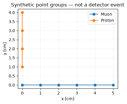
Try: explain why this plot alone cannot identify a muon or a proton. The labels came from our constructor arguments, not the displayed geometry.
3. Assemble and inspect an interaction
Narration transcript · draft
Now step up one level and collect the two candidates into an interaction. This helper assembles the objects we give it; it does not discover that they belong together. Compare the full particle list with the primary particle list, then read the topology summary. That distinction will matter whenever you turn an object collection into an analysis selection.
RecoInteraction.from_particles aggregates the supplied particles. It does
not run clustering, discover an interaction, or fit a vertex. We already chose
the association. We explicitly assign the interaction ID afterward.
interaction = RecoInteraction.from_particles(particles)
interaction.id = 0
print("Particle IDs:", interaction.particle_ids.tolist())
print("Primary IDs:", interaction.primary_particle_ids.tolist())
print("Number of particles:", interaction.num_particles)
print("Primary topology:", interaction.topology)
assert interaction.num_particles == 2
assert interaction.num_primary_particles == 2
assert interaction.size == 10
Particle IDs: [0, 1]
Primary IDs: [0, 1]
Number of particles: 2
Primary topology: 1mu1p
The topology string summarizes valid primary particles by species. It is
not the complete particle inventory or an interaction-mode classification.
The particles collection is still available when you need individual objects.
Missing estimates such as an unfitted vertex must not be interpreted as measurements.
Try: use interaction.particles to print the size of each constituent.
Before running it, predict whether the two sizes add up to interaction.size.
They do for this disjoint fixture; do not assume arbitrary manually assembled
collections satisfy that invariant.
4. Turn an object inspection into a small analysis
Narration transcript · draft
Before running the last example, predict what changes when we remove one primary flag. The points stay exactly where they were, and both particles still exist, but the primary topology changes. This is a useful habit for analysis: say precisely what your selection counts. Later, when you read real HDF5 output, bring the same care to labels, units, and production settings.
A selection should state precisely what it counts. Below we count primary muon candidates. This is a reconstructed selection, not a claim that the event is a particular neutrino interaction or that the particle identification is accurate.
primary_muons = [
    particle
    for particle in interaction.particles
    if particle.is_primary and particle.is_valid and particle.pid == MUON_PID
]
print("Valid primary muon candidates:", len(primary_muons))
assert len(primary_muons) == 1

# Controlled experiment: change a classification, then rebuild the aggregate.
modified = deepcopy(particles)
modified[1].is_primary = False
alternate = RecoInteraction.from_particles(modified)
print("After changing only the proton primary flag:")
print(
    "particles =",
    alternate.num_particles,
    "; primaries =",
    alternate.num_primary_particles,
    "; topology =",
    alternate.topology,
)
assert alternate.num_particles == 2
assert alternate.num_primary_particles == 1
assert alternate.size == interaction.size
Valid primary muon candidates: 1
After changing only the proton primary flag:
particles = 2 ; primaries = 1 ; topology = 1mu
Exercise: change the muon’s primary flag instead. Predict the primary-muon count and topology before executing. Then restore the original fixture by running the notebook from the top. No point moved; only a classification changed.
You can now separate three questions: what points belong to a candidate?,
what labels does it carry?, and how are candidates associated? With a real
SPINE production, the next step is to read its output and inspect the same
objects, while recording the software version, configuration, units, and
calibration. Reading HDF5 and interpreting energy loss (dE/dx) are later lessons.
References and next steps
The wider ecosystem includes DUNE and ICARUS applications, UResNet and Graph-SPICE reconstruction components, and sparse-convolution tooling such as MinkowskiEngine. None is required to run this object-inspection lesson.